Getting Started with risdr • risdr

Purpose

Sufficient dimension reduction seeks a low-dimensional projection \mathbf{B}^{\mathsf{T}}\mathbf{X} that retains the information in the predictors \mathbf{X} about a response Y. The working condition is

$Y \perp\!\!\!\perp \mathbf{X}\mid \mathbf{B}^{\mathsf{T}}\mathbf{X}.$

risdr combines classical inverse-regression estimators with covariance regularisation, structural dimension criteria, prediction, and resampling. The implemented SDR methods are SIR (Li 1991), SAVE (Cook 1998), DR (Li and Wang 2007), and pHd (Li 1992).

A reproducible example

library(risdr)

sim <- simulate_risdr_data(
  n = 160,
  p = 20,
  d = 2,
  rho = 0.6,
  sigma = 0.7,
  model = "linear_quadratic",
  seed = 2026
)

The simulation object contains the predictor matrix, response, true central subspace basis, sufficient predictors, population covariance matrix, signal, noise, and generation settings.

str(sim[c("X", "y", "beta", "Sigma", "n", "p", "d")], max.level = 1)
#> List of 7
#>  $ X    : num [1:160, 1:20] 0.693 -0.258 0.472 -0.714 -0.621 ...
#>   ..- attr(*, "dimnames")=List of 2
#>  $ y    : num [1:160] 0.6767 2.2458 0.0652 1.7558 0.0142 ...
#>  $ beta : num [1:20, 1:2] -1 0 0 0 0 0 0 0 0 0 ...
#>   ..- attr(*, "dimnames")=List of 2
#>  $ Sigma: num [1:20, 1:20] 1 0.6 0.36 0.216 0.13 ...
#>  $ n    : int 160
#>  $ p    : int 20
#>  $ d    : int 2

Fit an SDR model

fit <- fit_risdr(
  X = sim$X,
  y = sim$y,
  sdr_method = "dr",
  cov_method = "oas",
  nslices = 6,
  d_max = 6,
  selector = "cicomp",
  standardize = TRUE,
  stabilize = TRUE
)

fit
#> Regularised and Information-Theoretic SDR fit
#> --------------------------------------------------
#> SDR method       : DR 
#> Covariance       : OAS 
#> Stabilised       : TRUE 
#> Stabilisation    : eigenfloor 
#> Selected d       : 1 
#> Selector         : CICOMP 
#> Number of slices : 6 
#> Observations     : 160 
#> Predictors       : 20
summary(fit)
#> Summary of risdr fit
#> --------------------------------------------------
#> Method              : DR 
#> Covariance          : OAS 
#> Selected dimension  : 1 
#> Selector            : CICOMP 
#> 
#> Leading eigenvalues:
#>  [1] 3.546972 2.413215 2.342954 1.760832 1.678750 1.613520 1.544909 1.470014
#>  [9] 1.379194 1.318532
#> 
#> Dimension selection table:
#>   d      AIC      BIC     CAIC    ICOMP   CICOMP
#> 1 1 652.4135 661.6390 664.6390 646.4136 664.6392
#> 2 2 648.6741 660.9748 664.9748 640.6798 664.9805
#> 3 3 645.1711 660.5470 665.5470 635.1832 665.5591
#> 4 4 643.7799 662.2309 668.2309 631.7938 668.2448
#> 5 5 643.1144 664.6406 671.6406 629.1346 671.6608
#> 6 6 644.7628 669.3642 677.3642 628.7866 677.3880
#> 
#> Covariance diagnostics:
#> $min_eigenvalue
#> [1] 0.2571752
#> 
#> $max_eigenvalue
#> [1] 3.881756
#> 
#> $condition_number
#> [1] 15.09382
#> 
#> $effective_rank
#> [1] 20

The fitted object stores the training transformations, covariance estimate, kernel, eigenvalues, directions, scores, dimension-selection table, and downstream linear model.

Inspect the structural dimension

fit$d_table
#>   d      AIC      BIC     CAIC    ICOMP   CICOMP
#> 1 1 652.4135 661.6390 664.6390 646.4136 664.6392
#> 2 2 648.6741 660.9748 664.9748 640.6798 664.9805
#> 3 3 645.1711 660.5470 665.5470 635.1832 665.5591
#> 4 4 643.7799 662.2309 668.2309 631.7938 668.2448
#> 5 5 643.1144 664.6406 671.6406 629.1346 671.6608
#> 6 6 644.7628 669.3642 677.3642 628.7866 677.3880
criterion_weights(fit$d_table, criterion = "CICOMP")
#>   d criterion    value      delta       weight
#> 1 1    CICOMP 664.6392  0.0000000 0.3744185043
#> 2 2    CICOMP 664.9805  0.3413617 0.3156687272
#> 3 3    CICOMP 665.5591  0.9199146 0.2363743701
#> 4 4    CICOMP 668.2448  3.6056768 0.0617155391
#> 5 5    CICOMP 671.6608  7.0216670 0.0111846317
#> 6 6    CICOMP 677.3880 12.7488687 0.0006382277

Information criteria answer a model-selection question, while predictive cross-validation estimates out-of-fold error. Both should be considered when the selected dimension is consequential.

cv <- select_dimension_cv(
  X = sim$X,
  y = sim$y,
  sdr_method = "dr",
  cov_method = "oas",
  d_max = 5,
  v = 5,
  nslices = 6,
  metric = "RMSE",
  seed = 2026
)

cv$selected_d
#> [1] 4
cv$cv_table
#>   d     RMSE      MAE     MAPE         R2  Adjusted_R2 Correlation   RMSE_SD
#> 1 1 1.925508 1.320080 401.7670 0.02811421 -0.004281982   0.3532172 0.3417961
#> 2 2 1.914872 1.303977 403.1347 0.05440990 -0.010803214   0.3706750 0.3731576
#> 3 3 1.913670 1.261976 383.4571 0.04526626 -0.057026641   0.3479463 0.3251972
#> 4 4 1.882636 1.241811 368.9813 0.07647568 -0.060342736   0.3744047 0.3206029
#> 5 5 1.885588 1.229950 356.3241 0.07431750 -0.103698361   0.3746814 0.3111336
#>      MAE_SD  MAPE_SD     R2_SD Adjusted_R2_SD Correlation_SD
#> 1 0.1579465 218.8750 0.2886675      0.2982898      0.2784702
#> 2 0.1921951 217.5938 0.2265393      0.2421626      0.2340298
#> 3 0.1659905 213.1066 0.2454981      0.2718015      0.2139119
#> 4 0.1754700 229.4375 0.2390968      0.2745185      0.2026659
#> 5 0.1675317 216.1027 0.2329199      0.2777122      0.1938162

Prediction

Prediction applies the training centre, scale, SDR centre, and estimated directions to new observations before invoking the downstream model.

predicted <- predict(fit, sim$X[1:12, , drop = FALSE])
evaluate_prediction(
  y_true = sim$y[1:12],
  y_pred = predicted,
  d = fit$d
)
#>       RMSE      MAE     MAPE        R2 Adjusted_R2 Correlation
#> 1 1.579152 1.165364 1161.818 0.4183239   0.3601562   0.6936867

Named columns may be supplied in a different order. They are checked and reordered to the training layout. A single new observation is also valid.

Component-specific controls

Arguments for covariance estimation, covariance stabilisation, and SDR kernels are supplied separately. This prevents a control intended for one component from being passed to another component.

fit_ridge <- fit_risdr(
  X = sim$X,
  y = sim$y,
  sdr_method = "sir",
  cov_method = "ridge",
  d = 2,
  d_max = 5,
  cov_args = list(lambda = 0.15),
  stabilization_args = list(eps = 1e-7),
  sdr_args = list(slice_type = "quantile")
)

Diagnostics

plot_scree(fit, n_eigen = 10)
plot_sufficient(fit, direction = 1)
plot_dimension_selection(fit)

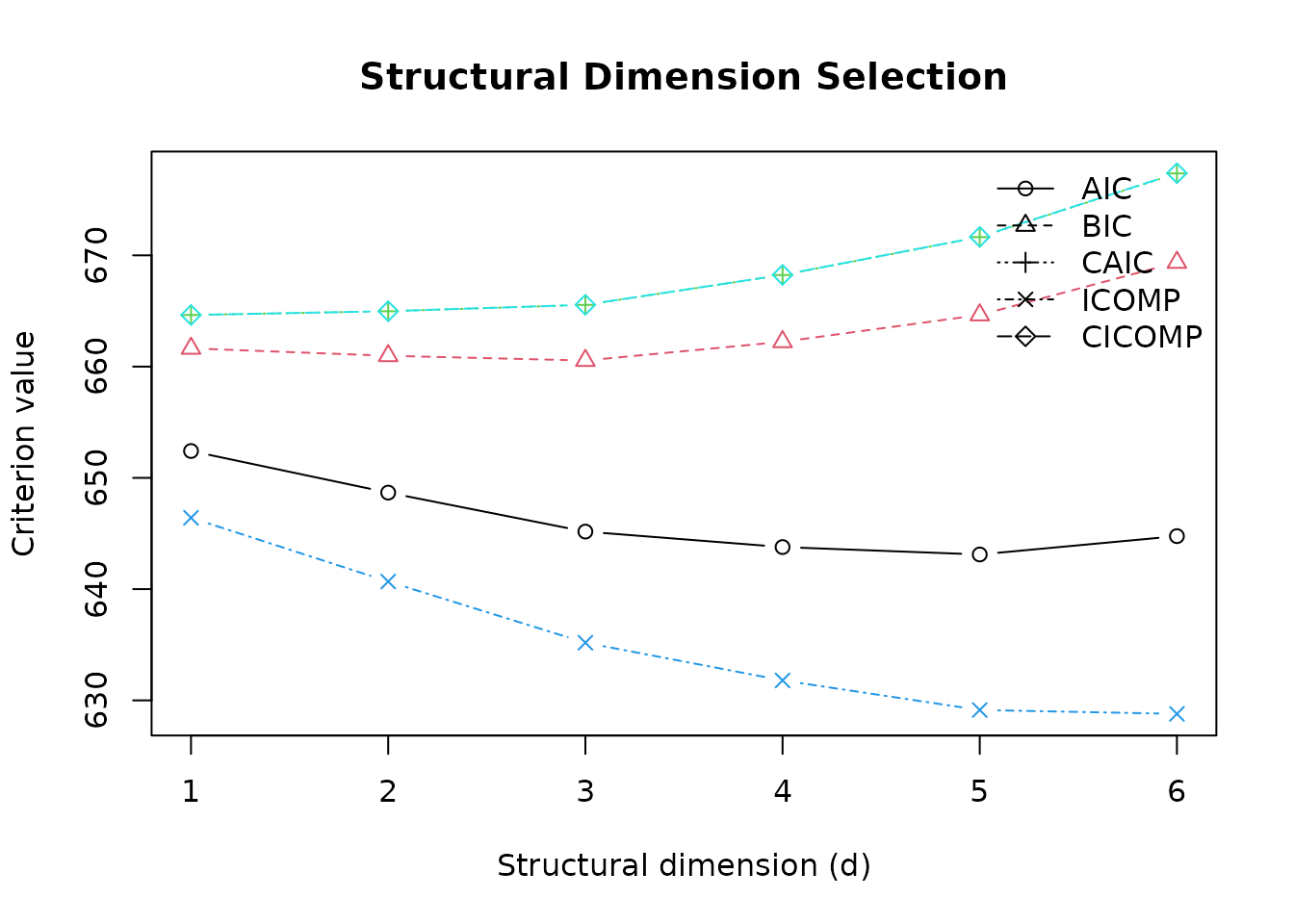
Loadings and sufficient summary plots are descriptive. Signs of eigenvectors are not identified, so sign reversals across numerically equivalent fits do not change the estimated subspace.

Current scope

The verified modelling interface is for continuous responses. The standalone MEC covariance helper accepts additional working response forms, but binary, multiclass, and censored survival modelling are not yet claimed as complete risdr workflows.

References

Cook, R. Dennis. 1998. Regression Graphics: Ideas for Studying Regressions Through Graphics. Wiley. https://doi.org/10.1002/9780470316931.

Li, Bing, and Shaoli Wang. 2007. “On Directional Regression for Dimension Reduction.” Journal of the American Statistical Association 102 (479): 997–1008. https://doi.org/10.1198/016214507000000536.

Li, Ker-Chau. 1991. “Sliced Inverse Regression for Dimension Reduction.” Journal of the American Statistical Association 86 (414): 316–27. https://doi.org/10.1080/01621459.1991.10475035.

Li, Ker-Chau. 1992. “On Principal Hessian Directions for Data Visualization and Dimension Reduction: Another Application of Stein’s Lemma.” Journal of the American Statistical Association 87 (420): 1025–39. https://doi.org/10.1080/01621459.1992.10476258.